Dermatitis
The UCI data set (Ilter and Altay Güvenir 1998) consist of
- \(366\) patients (\(8\) with missing values)
- \(12\) clinical attributes (erythema, itching, scaling, etc.)
- \(21\) histopathological attributes (decrease of melanin, spongiosis, etc.)
and a class variable with six different skin diseases
- psoriasis (\(111\) patients)
- seborrheic dermatitis (\(60\) patients)
- lichen planus (\(71\) patients)
- pityriasis rosea (\(48\) patients)
- chronic dermatitis (\(48\) patients)
- pityriasis rubra pilaris (\(20\) patients)
Many of the classical machine learning algorithms have been applied to the dataset (Liu et al. 2015). They all achieve a prediction accuracy above \(95\%\) and some even above \(99\%\). But…:
- The skin diseases share many common features
- We have exclusive classes but possibly not exhaustive
- What if a patient does not suffer from one of the six diseases
- Classification forces us to label a patient with one and only one disease
Goal
Given a new patient \(y\), we want to test the hypotheses
\[\begin{align*} H_1: & y \text{ has psoriasis} \\ H_2: & y \text{ has seborrheic dermatitis} \\ H_3: & y \text{ has lichen planus} \\ H_4: & y \text{ has pityriasis rosea} \\ H_5: & y \text{ has chronic dermatitis} \\ H_6: & y \text{ has pityriasis rubra pilaris} \end{align*}\]Since all hypotheses are exclusive we do not correct for multiple hypothesis testing (but the user can do this by setting the significance level accordingly).
Modeling Attributes of Psoriasis
We first show how to test \(H_1\). First extract the psoriasis data:
library(dplyr)
library(molic)
y     <- unlist(derma[80, -35]) # a patient with seboreic dermatitis
psor  <- derma %>%
  filter(ES == "psoriasis") %>%
  dplyr::select(-ES)
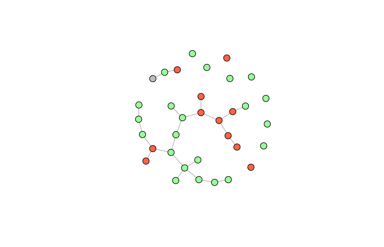
Next, we fit the interaction graph for the psoriasis patients:
We can color the nodes corresponding to clinical attributes (red), histopathological attributes (green) and the age variable (gray):
vs   <- names(adj_lst(g))
vcol <- structure(vector("character", length(vs)), names = vs)
vcol[grepl("c", vs)] <- "tomato"  # clinical attributes
vcol[grepl("h", vs)] <- "#98FB98" # histopathological attributes
vcol["age"]          <- "gray"    # age variable
plot(g, vcol, vertex.size = 10, vertex.label = NA)

The take home message here is, that we cannot assume independence between the attributes for the psoriasis patient as seen in the interaction graph - there are many associations.
Outlier Model for Psoriasis Patients
set.seed(300718)
m <- fit_outlier(psor, g, y)
print(m)
 --------------------------------
  Simulations: 10000
  Variables: 34
  Observations: 112
  Estimated mean: 42.66
  Estimated variance: 37.55
 --------------------------------
  Critical value: 53.86771
  Deviance: 50.51582
  P-value: 0.1053
  Alpha: 0.05
  <novelty, outlier_model, list>
 --------------------------------
Notice that that the number of observations is \(112\) even though we have only observed \(111\) psoriasis patients. This is because, under the hypothesis, \(H_1\), the new observation \(y\) has psoriasis. The other summary statistics is self explanatory.
Plotting the Approximated Density of the Test Statistic
plot(m)
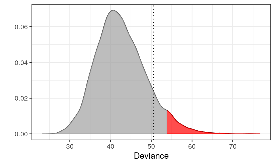
 The red area is the critical region (here 5%) and the dotted line is the observed test statistic (the deviance) of \(y\). Since the dotted line is outside the critical region, we cannot reject that \(y\) has psoriasis.
Testing all Hypothesis Simultaneously
We can use the fit_multiple_models function to test all six hypothesis as follows.
set.seed(300718)
mm <- fit_multiple_models(derma, y, "ES", q = 0,trace = FALSE)
plot(mm)

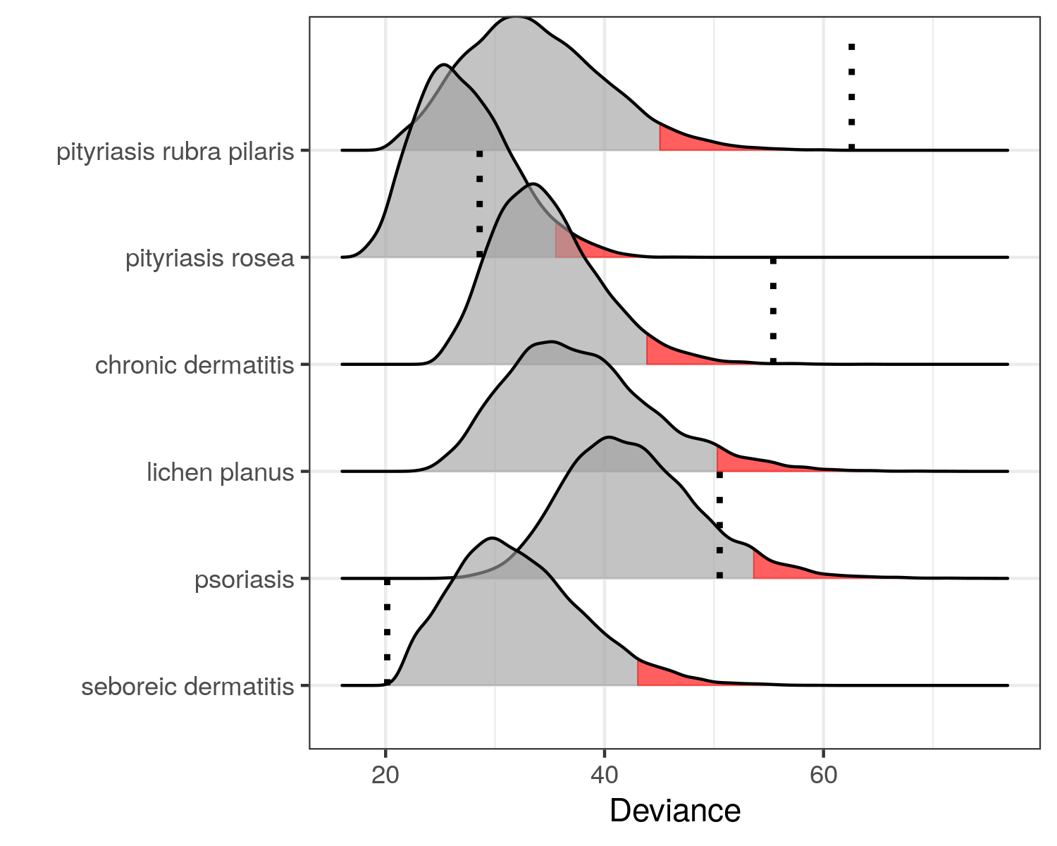
Thus, we cannot reject that \(y\) has either psoriasis, seboreic dermatitis or pityriasis rosea. This is conservative compared to classification methods and hence a little safer. The medical expert should proceed the investigation from here.
References
Ilter, and H. Altay Güvenir. 1998. “UCI Machine Learning Repository.” Department of Computer Engineering; Information Science. https://archive.ics.uci.edu/ml/datasets/Dermatology.
Liu, Tong, Liang Hu, Chao Ma, Zhi-Yan Wang, and Hui-Ling Chen. 2015. “A Fast Approach for Detection of Erythemato-Squamous Diseases Based on Extreme Learning Machine with Maximum Relevance Minimum Redundancy Feature Selection.” International Journal of Systems Science 46 (5). Taylor & Francis: 919–31.