Outlier Detection in Genetic Data
Mads Lindskou
Source:vignettes/genetic_example.Rmd
genetic_example.RmdThe 1000 Genomes Project Data
The outlier detection method (Lindskou, Svante Eriksen, and Tvedebrink 2019) arose from a problem in the forensic science community where it is of great interest to make statements about the geographical origin of a DNA sample. This is in general a very complicated matter. More over, when DNA markers are in linkage disequilibrium things get even more complicated. The 1000 Genomes Project set out to provide a comprehensive description of common human genetic variation by applying whole-genome sequencing to a diverse set of individuals from multiple populations (The 1000 Genomes Project Consortium 2015). In the molic package we include the final data from the project which includes \(2504\) DNA profiles coming from five different continental regions; Europe (EUR), Africa (AFR), America (AMR), East Asia (EAS), South Asia (SAS). Each DNA profile is the compound of two rows in the data tgp_dat, one for each chromosome copy. This makes the outlier procedure slightly more complicated since we must fit a model to each copy and aggregate the information (but we shall see in a moment that it is not hard to do using the molic package).
The data includes \(276\) SNP markers grouped in \(97\) microhaplotypes; in other words, the SNPs within a microhaplotype are so close that they cannot be assumed to be in linkage disequilibrium and we must take into account their mutual dependencies. We do this with the use of decomposable graphical models. See the outlier_intro for more details on the model. The microhaplotype grouping is provided is the list tgp_haps.
Setup and Data
library(molic)
library(ess)   # for fit_components
library(dplyr)
set.seed(7)    # for reproducibility

## Data

# The components - here microhaplotypes
haps <- tgp_haps

# All the Europeans
eur <- tgp_dat %>%
  as_tibble() %>%
  filter(pop_meta == "EUR")

# Extracting the two databases for each copy of the chromosomes
eur_a <- eur %>%
  filter(grepl("a$", sample_name)) %>%
  select(-c(1:2))

eur_b <- eur %>%
  filter(grepl("b$", sample_name)) %>%
  select(-c(1:2))
We peak at data:
print(eur, n_extra = 0)
## # A tibble: 1,006 x 304
##    sample_name pop_meta rs28529526 rs10134526 rs260694 rs11123719 rs11691107
##    <chr>       <chr>    <chr>      <chr>      <chr>    <chr>      <chr>
##  1 HG00096a    EUR      G          C          T        T          C
##  2 HG00097a    EUR      G          T          T        C          C
##  3 HG00099a    EUR      G          C          T        T          C
##  4 HG00100a    EUR      G          C          T        T          C
##  5 HG00101a    EUR      G          C          T        T          C
##  6 HG00102a    EUR      G          C          T        T          C
##  7 HG00103a    EUR      G          C          T        C          C
##  8 HG00105a    EUR      G          T          T        C          C
##  9 HG00106a    EUR      G          C          T        C          C
## 10 HG00107a    EUR      G          C          T        T          C
## # … with 996 more rows, and 297 more variables
We now fit the interaction graphs for each chromosome copy. We use fit_components since we know, that SNPs between haplotypes are independent. This also makes the procedure much faster.
ga <- fit_components(eur_a, comp = haps, trace = FALSE)
gb <- fit_components(eur_b, comp = haps, trace = FALSE)
print(ga)
##  A Decomposable Graph With
##  -------------------------
##   Nodes: 302
##   Edges: 234 / 45451
##   Cliques: 161
##    - max: 4
##    - min: 1
##    - avg: 2.18
##   <gengraph, list>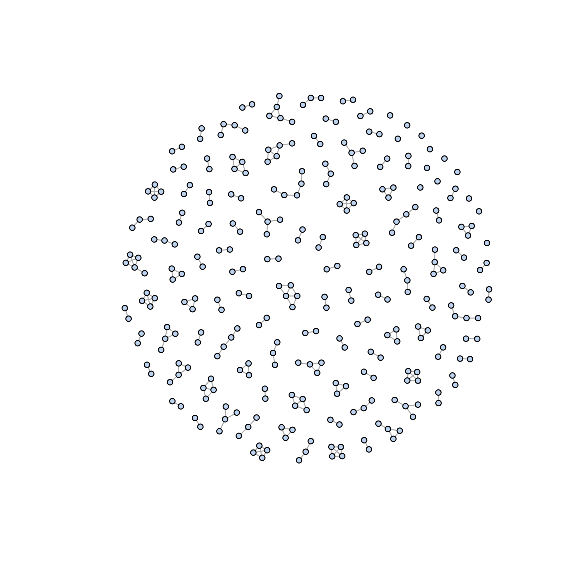
## -------------------------plot(ga, vertex.size = 3, vertex.label = NA)
Example 1 - Testing which observations within data are outliers
Fitting the model:
# Only 500 simulations is used here to exeplify
# The default number of simulations is 10,000
m1 <- fit_outlier(eur_a, ga, nsim = 500) # consider using more cores (ncores argument)
m2 <- fit_outlier(eur_b, gb, nsim = 500) # consider using more cores (ncores argument)
m  <- fit_mixed_outlier(m1, m2)
Model information:
print(m)
##
## --------------------------------
## Simulations: 500
## Variables: 302
## Observations: 503
## Estimated mean: 482.36
## Estimated variance: 345.85
## --------------------------------
## Critical value: 516.8367
## Alpha: 0.05
## <mixed_outlier, outlier, outlier_model, list>
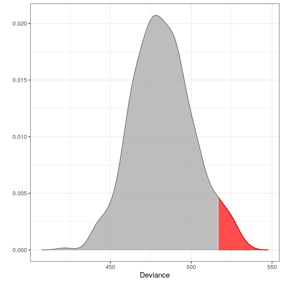
## --------------------------------The distribution of the test statistic:
plot(m)
Locating the outliers:
outs <- outliers(m)
eur_a_outs <- eur_a[which(outs), ]
eur_b_outs <- eur_b[which(outs), ]
print(eur_a_outs, n_extra = 0)
## # A tibble: 19 x 302
##    rs28529526 rs10134526 rs260694 rs11123719 rs11691107 rs12469721 rs3101043
##    <chr>      <chr>      <chr>    <chr>      <chr>      <chr>      <chr>
##  1 G          C          T        T          C          A          C
##  2 G          C          T        C          C          T          T
##  3 G          C          T        T          C          T          T
##  4 G          C          T        C          C          A          T
##  5 G          T          T        T          C          A          T
##  6 G          C          T        C          C          T          T
##  7 G          T          T        T          C          A          C
##  8 G          C          T        C          C          A          C
##  9 G          C          T        T          C          A          C
## 10 G          C          T        C          C          T          C
## 11 G          C          T        T          C          T          C
## 12 G          C          T        C          C          A          T
## 13 G          C          T        T          C          T          T
## 14 G          C          T        T          T          T          T
## 15 G          C          T        T          C          A          C
## 16 G          C          T        T          C          T          T
## 17 G          C          T        T          C          T          C
## 18 G          T          T        T          C          T          C
## 19 G          T          T        T          C          A          T
## # … with 295 more variables
Retrieving the deviance test statistic for individual observations:
x1 <- rbind(eur_a_outs[1, ], eur_b_outs[1, ])
x2 <- rbind(eur_a[1, ], eur_b[1, ])
dev1 <- deviance(m, x1) # falls within the critical region in the plot (the red area)
dev2 <- deviance(m, x2) # falls within the acceptable region in the plot

dev1
## [1] 537.9733dev2## [1] 496.799# Retrieving the pvalues pval(m, dev1)
## [1] 0pval(m, dev2)
## [1] 0.208Example 2 - Testing if a new observation is an outlier
Testing if an American is an outlier in Europe:
amr <- tgp_dat %>%
  as_tibble() %>%
  filter(pop_meta == "AMR")

z1  <- amr %>%
  filter(grepl("a$", sample_name)) %>%
  select(unname(unlist(haps))) %>%
  slice(1) %>%
  unlist()

z2  <- amr %>%
  filter(grepl("b$", sample_name)) %>%
  select(unname(unlist(haps))) %>%
  slice(1) %>%
  unlist()

# Only 500 simulations is used here to exemplify
# The default number of simulations is 10,000
m3 <- fit_outlier(eur_a, ga, z1, nsim = 500) # consider using more cores (ncores argument)
m4 <- fit_outlier(eur_b, gb, z2, nsim = 500) # consider using more cores (ncores argument)
m5 <- fit_mixed_outlier(m3, m4)
print(m5)
##
##  --------------------------------
##   Simulations: 500
##   Variables: 302
##   Observations: 504
##   Estimated mean: 483.14
##   Estimated variance: 341.9
##  --------------------------------
##   Critical value: 516.6007
##   Deviance: 508.0499
##   P-value: 0.098
##   Alpha: 0.05
##   <mixed_outlier, novelty, outlier_model, list>
## --------------------------------plot(m5)
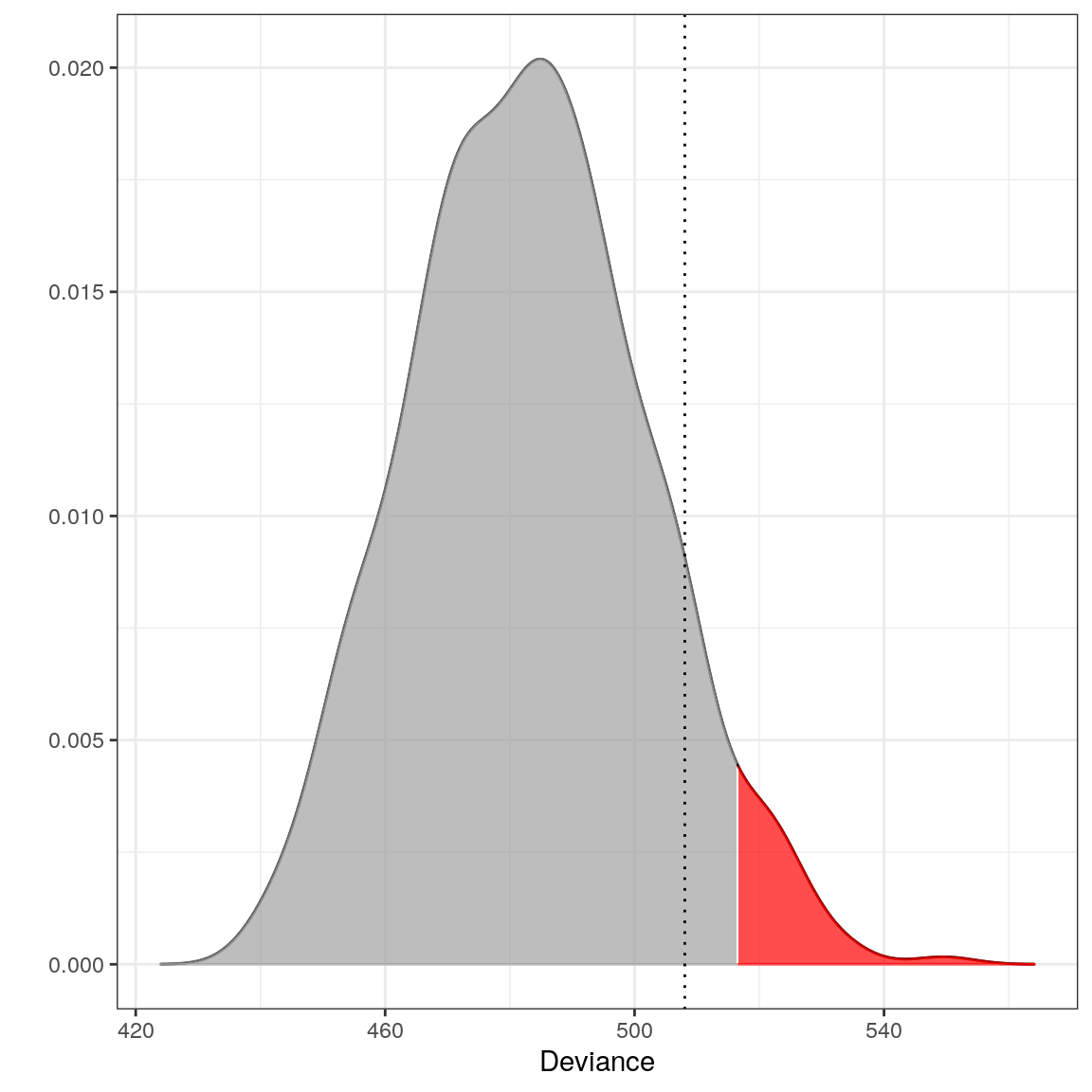
Thus, z does not deviate significantly from the Europe database. The red area depicts the \(0.05\) significance level and the dotted line is the observed deviance of z (508.0498712). This is not a complete surprise, since Americans and Europeans have many similarities.
References
Lindskou, Mads, Poul Svante Eriksen, and Torben Tvedebrink. 2019. “Outlier Detection in Contingency Tables Using Decomposable Graphical Models.” Scandinavian Journal of Statistics. Wiley Online Library. doi:10.1111/sjos.12407.
The 1000 Genomes Project Consortium. 2015. “A Global Reference for Human Genetic Variation.” Nature 526 (7571). Nature Publishing Group: 68. doi:10.1038/nature15393.