Mixed Outlier Test

A function for outlier detection with mixed, but independen, information

fit_mixed_outlier(m1, m2)

Arguments

m1	An object returned from fit_outlier
m2	An object returned from fit_outlier

Value

An object of type mixed_outlier with novelty or outlier as child classes. These are used for different purposes. See fit_outlier.

Details

It is assumed that the input data to m1 and m2 holds information about the same observation in corresponding rows. Thus, the two datasets must also be of same dimension.

See also

fit_outlier, fit_multiple_models, outliers, pval, deviance

Examples

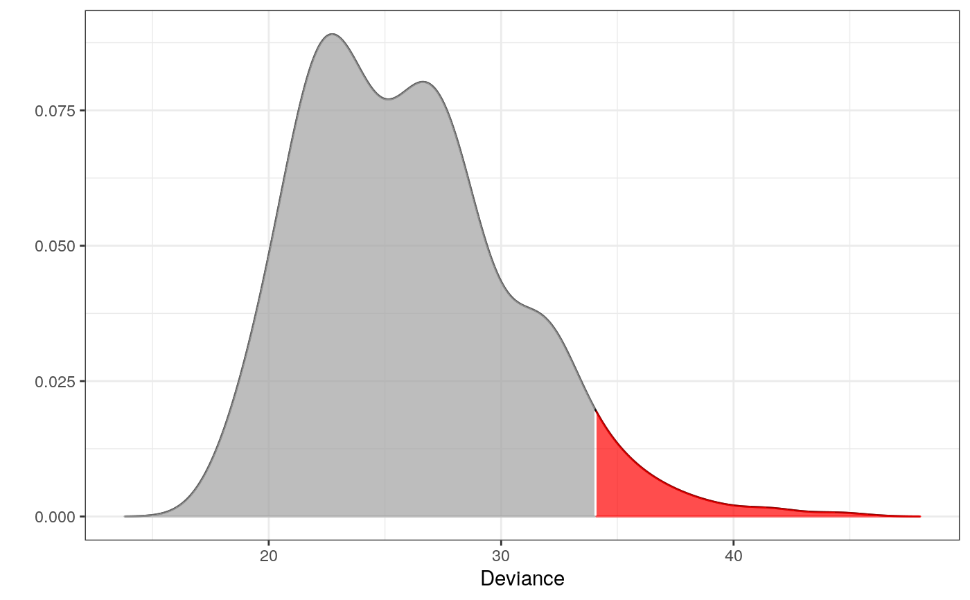
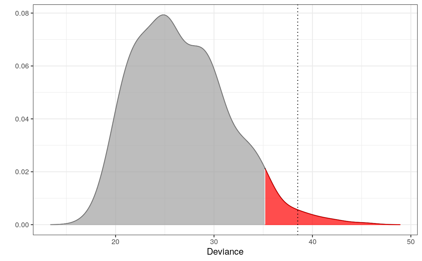
library(dplyr)
#> 
#> Attaching package: ‘dplyr’
#> The following objects are masked from ‘package:stats’:
#> 
#>     filter, lag
#> The following objects are masked from ‘package:base’:
#> 
#>     intersect, setdiff, setequal, union
library(ess)  # for fit_components
#> Registered S3 method overwritten by 'ess':
#>   method     from
#>   print.tree cli 
set.seed(7)   # for reproducibility

## Data

# The components - here microhaplotypes
haps <- tgp_haps[1:5] # only a subset of data is used to exemplify
dat <- tgp_dat %>%
       select(pop_meta, sample_name, all_of(unname(unlist(haps))))

# All the Europeans
eur <- dat %>%
  as_tibble() %>%
  filter(pop_meta == "EUR")

# Extracting the two databases for each copy of the chromosomes
eur_a <- eur %>%
  filter(grepl("a$", sample_name)) %>%
  select(-c(1:2))

eur_b <- eur %>%
  filter(grepl("b$", sample_name)) %>%
  select(-c(1:2))


# Fitting the interaction graphs on the EUR data 
ga <- fit_components(eur_a, comp = haps, trace = FALSE)
gb <- fit_components(eur_b, comp = haps, trace = FALSE)
print(ga)
#>  A Decomposable Graph With 
#>  ------------------------- 
#>   Nodes: 17 
#>   Edges: 18 / 136 
#>   Cliques: 7 
#>    - max: 4 
#>    - min: 1 
#>    - avg: 2.57 
#>   <gengraph, list> 
#>  -------------------------
plot(ga, vertex.size = 1)

## ---------------------------------------------------------
##                       EXAMPLE 1
##   Testing which observations within data are outliers
## ---------------------------------------------------------

# Only 500 simulations is used here to exeplify
# The default number of simulations is 10,000
m1 <- fit_outlier(eur_a, ga, nsim = 500) # consider using more cores (ncores argument)
m2 <- fit_outlier(eur_b, gb, nsim = 500) # consider using more cores (ncores argument)
m  <- fit_mixed_outlier(m1, m2)
print(m)
#> 
#>  -------------------------------- 
#>   Simulations: 500 
#>   Variables: 17 
#>   Observations: 503 
#>   Estimated mean: 25.95 
#>   Estimated variance: 20.47 
#>  --------------------------------
#>   Critical value: 34.03098 
#>   Alpha: 0.05 
#>   <mixed_outlier, outlier, outlier_model, list> 
#>  --------------------------------
plot(m)

outs <- outliers(m)
eur_a_outs <- eur_a[which(outs), ]
eur_b_outs <- eur_b[which(outs), ]

# Retrieving the test statistic for individual observations
x1 <- rbind(eur_a_outs[1, ], eur_b_outs[1, ])
x2 <- rbind(eur_a[1, ], eur_b[1, ])
dev1 <- deviance(m, x1) # falls within the critical region in the plot (the red area)
dev2 <- deviance(m, x2) # falls within the acceptable region in the plot

dev1
#> [1] 39.01466
dev2
#> [1] 27.03032

# Retrieving the pvalues
pval(m, dev1)
#> [1] 0.008
pval(m, dev2)
#> [1] 0.372


# \donttest{

## ---------------------------------------------------------
##                       EXAMPLE 2
##      Testing if a new observation is an outlier
## ---------------------------------------------------------

# Testing if an American is an outlier in Europe
amr <- dat %>%
  as_tibble() %>%
  filter(pop_meta == "AMR")

z1  <- amr %>%
  filter(grepl("a$", sample_name)) %>%
  select(unname(unlist(haps))) %>%
  slice(1) %>%
  unlist()

z2  <- amr %>%
  filter(grepl("b$", sample_name)) %>%
  select(unname(unlist(haps))) %>%
  slice(1) %>%
  unlist()

# Only 500 simulations is used here to exemplify
# The default number of simulations is 10,000
m3 <- fit_outlier(eur_a, ga, z1, nsim = 500) # consider using more cores (ncores argument)
m4 <- fit_outlier(eur_b, gb, z2, nsim = 500) # consider using more cores (ncores argument)
m5 <- fit_mixed_outlier(m3, m4)
print(m5)
#> 
#>  -------------------------------- 
#>   Simulations: 500 
#>   Variables: 17 
#>   Observations: 504 
#>   Estimated mean: 26.74 
#>   Estimated variance: 22.3 
#>  --------------------------------
#>   Critical value: 35.1841 
#>   Deviance: 38.50607 
#>   P-value: 0.016 
#>   Alpha: 0.05 
#>   <mixed_outlier, novelty, outlier_model, list> 
#>  --------------------------------
plot(m5)

# }